Experiment: Study of Active Filter Circuits
1. Aim
To study the frequency and phase response of an active band-pass filter built around an operational amplifier, to measure the voltage gain as a function of frequency, to identify the resonant (centre) frequency, and to automate the frequency sweep using a Python program.
2. Apparatus / Components Required
- SEELab3 or ExpEYES-17 unit
- Resistors: $R_1 = 10\text{ k}\Omega$, $R_2 = 1\text{ k}\Omega$, $R_3 = 100\text{ k}\Omega$
- Capacitors: $C_1 = 0.1\text{ }\mu F$, $C_2 = 0.01\text{ }\mu F$
- Operational Amplifier: OP07 (or equivalent precision op-amp) with $\pm 6\text{ V}$ supply
- Breadboard and connecting wires
- PC with Python 3 (libraries:
expeyes,numpy,scipy,matplotlib)
3. Theory & Principle
3.1 Filters
A filter is a circuit whose gain depends on the frequency of the input signal. The four basic types are:
- Low-pass filter (LPF): passes frequencies below a cut-off frequency $f_c$; attenuates higher frequencies.
- High-pass filter (HPF): passes frequencies above $f_c$; attenuates lower frequencies.
- Band-pass filter (BPF): passes a band of frequencies centred on a resonant frequency $f_0$; attenuates both below and above.
- Band-stop (Notch) filter: attenuates a specific narrow band of frequencies.
3.2 Active vs Passive Filters
A passive filter uses only R, L, C components. An active filter incorporates an operational amplifier, which provides gain, impedance buffering, and eliminates the loading effect between stages — allowing sharper and more controllable roll-off without the use of bulky inductors.
3.3 Voltage Gain and the Bode Plot
The voltage gain at each frequency is defined as:
\[A_v(f) = \frac{V_{out}(f)}{V_{in}(f)}\]Expressed in decibels (dB):
\[A_v\text{(dB)} = 20 \log_{10}\!\left(\frac{V_{out}}{V_{in}}\right)\]A plot of gain (dB) versus frequency on a logarithmic frequency axis is called a Bode plot. The frequency at which the gain drops to $\frac{1}{\sqrt{2}}$ of its peak value (i.e., $-3\text{ dB}$ below the peak) defines the bandwidth edges $f_1$ and $f_2$. The SEELab app plots the amplitude ratio of output and input signals vs frequency.
\[\text{Bandwidth} = f_2 - f_1\]3.4 The Designed Circuit
The active band-pass filter in this experiment uses an OP07 op-amp with the following component values:
| Component | Value |
|---|---|
| $R_1$ | $10\text{ k}\Omega$ |
| $R_2$ | $1\text{ k}\Omega$ |
| $R_3$ | $100\text{ k}\Omega$ |
| $C_1$ | $0.1\text{ }\mu F$ |
| $C_2$ | $0.01\text{ }\mu F$ |
The circuit was designed using the Okawa Online Filter Design Tool. The theoretical resonant frequency is:
\[f_0 = 527.8\text{ Hz}\]Design constraint: Choose component values such that the peak gain $A_v < 1$ (i.e., $< 0\text{ dB}$) to prevent output clipping. The WG frequency range of SEELab3/ExpEYES-17 is 5 Hz to 5000 Hz — all measurements must lie within this range.
3.5 Phase Response
In addition to amplitude, the output signal is phase-shifted relative to the input by an angle $\phi(f)$ that varies with frequency. At the resonant frequency of a band-pass filter, the phase shift is $0°$. Below $f_0$ the output leads the input; above $f_0$ it lags. Extracting phase requires fitting the time-domain waveforms to a sinusoidal model.
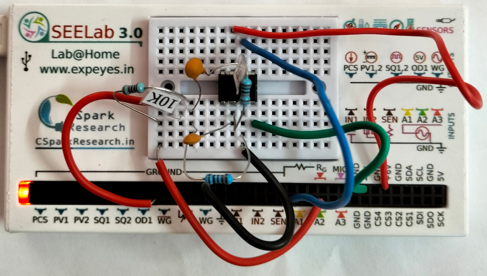
4. Circuit Diagram / Setup
- Assemble the active band-pass filter on a breadboard using the component values listed above. Refer to the schematic displayed in the SEELab3 app.
- Power the op-amp from the $\pm 12\text{ V}$ supply rails (or the available dual supply). Connect GND of the supply to the SEELab3 GND.
- WG → Filter input: Connect the Wave Generator output (WG) to both the filter input and channel A2 (to monitor $V_{in}$).
- Filter output → A2: Connect the op-amp output to channel A1 (to monitor $V_{out}$).
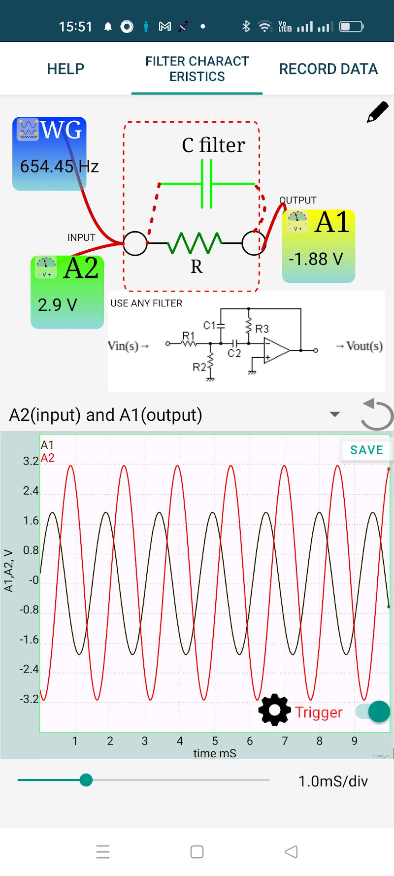
Steady State Response (Phone App)
Steady State Setup For ExpEYES17
5. Procedure
5a. Manual / App-Based Measurement
- Open the SEELab3 app and select the “Filter” experiment.
- Screen 1 — Waveform View: Set an initial frequency of $\approx 100\text{ Hz}$. The display shows $V_{in}$ (A1) and $V_{out}$ (A2) simultaneously. Slide vertically on the WG icon to change the frequency.
- Sweep the frequency from $\approx 100\text{ Hz}$ to $5000\text{ Hz}$ and observe how the output amplitude changes. Note the frequency at which $V_{out}$ is maximum — this is close to $f_0$.
- If output amplitude clips anywhere within the range, reduce input signal to 1V amplitude.
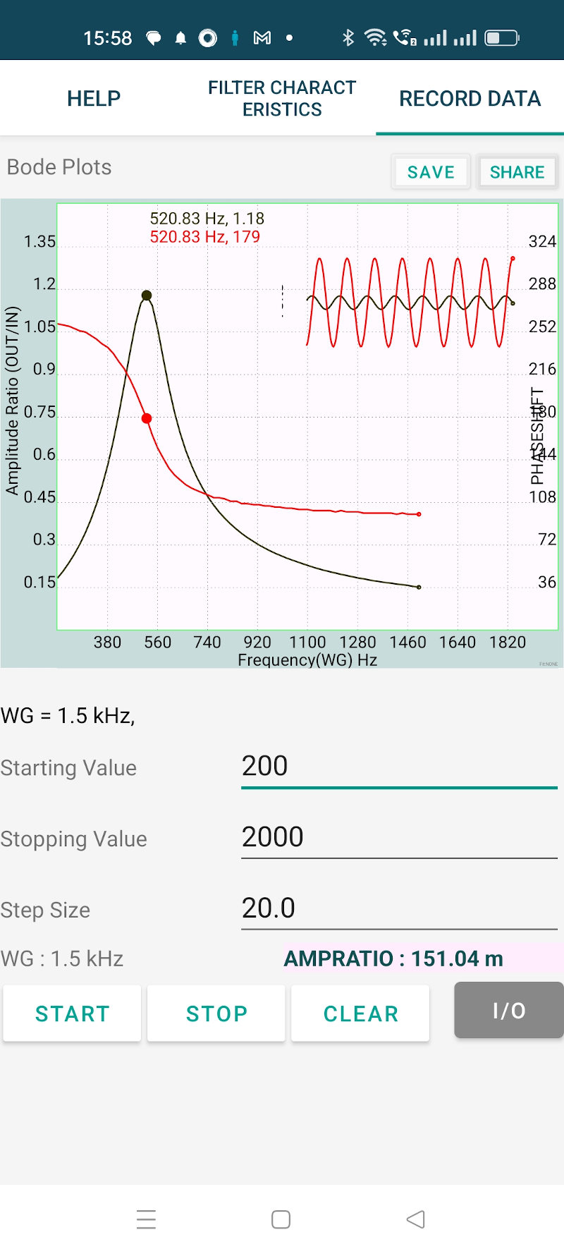
- Screen 2 — Record Data: Enter the start frequency, stop frequency, and step size. Click “Record”. The software automatically sweeps through all frequencies and plots:
- Gain plot: $A_v$ (or dB) vs $f$
- Phase plot: $\phi$ vs $f$
- Read off the peak frequency ($f_0$), the $-3\text{ dB}$ bandwidth edges ($f_1$, $f_2$), and the peak gain from the plot.
5b. Python Automation
The Python program replicates the manual sweep programmatically:
# filter-resp.py
# Measures voltage gain vs frequency and saves to CSV

import expeyes.eyesj as eyes
import numpy as np
import time

p = eyes.open()          # connect to SEELab3 / ExpEYES

start_freq  = 100        # Hz
stop_freq   = 5000       # Hz
step_freq   = 50         # Hz
amplitude   = 80         # WG amplitude (0–100 %)

results = []             # list to collect [freq, Vin, Vout, gain]

freq = start_freq
while freq <= stop_freq:
    p.set_sine(freq, amplitude)          # set WG frequency
    time.sleep(0.1)                      # allow signal to settle
    Vin  = p.get_voltage('A1')           # measure input amplitude
    Vout = p.get_voltage('A2')           # measure output amplitude
    gain = Vout / Vin if Vin != 0 else 0
    results.append([freq, Vin, Vout, gain])
    print(f"f={freq:5d} Hz  Vin={Vin:.3f}  Vout={Vout:.3f}  Gain={gain:.4f}")
    freq += step_freq

# Save data to CSV
with open('filter-resp.csv', 'w') as f:
    f.write('frequency,Vin,Vout,gain\n')
    for row in results:
        f.write(','.join(f'{v:.6f}' for v in row) + '\n')

print("Data saved to filter-resp.csv")
p.close()
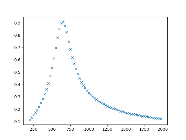
The analysis program reads the saved CSV and fits a Gaussian curve to the gain-frequency data to extract $f_0$ and bandwidth:
# filter-resp-analyse.py
# Reads CSV, plots frequency response, fits Gaussian to gain peak

import numpy as np
import matplotlib.pyplot as plt
from scipy.optimize import curve_fit

data = np.loadtxt('filter-resp.csv', delimiter=',', skiprows=1)
freq = data[:, 0]
gain = data[:, 3]

# Gaussian model: A * exp( -(f - f0)^2 / (2*sigma^2) )
def gaussian(f, A, f0, sigma):
    return A * np.exp(-0.5 * ((f - f0) / sigma) ** 2)

# Initial guesses
p0 = [max(gain), freq[np.argmax(gain)], 200]
popt, _ = curve_fit(gaussian, freq, gain, p0=p0)
A_fit, f0_fit, sigma_fit = popt

# -3 dB bandwidth: for Gaussian, BW ≈ 2 * sqrt(2*ln2) * sigma
bw = 2 * np.sqrt(2 * np.log(2)) * abs(sigma_fit)

print(f"Peak gain  : {A_fit:.4f}")
print(f"Centre freq: {f0_fit:.1f} Hz")
print(f"Bandwidth  : {bw:.1f} Hz")
print(f"Q factor   : {f0_fit / bw:.2f}")

plt.figure(figsize=(8, 4))
plt.plot(freq, gain, 'o', markersize=4, label='Measured')
plt.plot(freq, gaussian(freq, *popt), '-', label=f'Gaussian fit  $f_0$={f0_fit:.1f} Hz')
plt.axhline(A_fit / np.sqrt(2), color='gray', linestyle='--', label='-3 dB level')
plt.xlabel('Frequency (Hz)')
plt.ylabel('Voltage Gain $A_v$')
plt.title('Active Band-Pass Filter — Frequency Response')
plt.legend()
plt.grid(True, alpha=0.3)
plt.tight_layout()
plt.savefig('freq-resp.png', dpi=150)
plt.show()
6. Observation Table
| Theoretical $f_0$: $527.8\text{ Hz}$ | Measured $f_0$: ____ Hz |
6a. Manual Frequency Sweep
| Frequency $f$ (Hz) | $V_{in}$ (V) | $V_{out}$ (V) | Gain $A_v = V_{out}/V_{in}$ | Gain (dB) | Phase $\phi$ (°) |
|---|---|---|---|---|---|
| 100 | |||||
| 200 | |||||
| 350 | |||||
| 500 | |||||
| 528 | |||||
| 700 | |||||
| 1000 | |||||
| 2000 | |||||
| 5000 |
6b. Bandwidth and Quality Factor
| Quantity | Value |
|---|---|
| Peak gain $A_{v,\text{max}}$ | |
| Peak gain in dB | |
| $-3\text{ dB}$ level $= A_{v,\text{max}} / \sqrt{2}$ | |
| Lower $-3\text{ dB}$ frequency $f_1$ | |
| Upper $-3\text{ dB}$ frequency $f_2$ | |
| Bandwidth $\Delta f = f_2 - f_1$ | |
| Quality factor $Q = f_0 / \Delta f$ |
7. Results and Discussion
- The filter exhibited a band-pass characteristic with maximum gain at $f_0 =$ ____ Hz, against a theoretical value of $527.8\text{ Hz}$.
- The peak voltage gain was $A_{v,\text{max}} =$ ____ (____ dB), which is less than unity as designed.
- The $-3\text{ dB}$ bandwidth was found to be $\Delta f =$ ____ Hz, giving a quality factor $Q =$ ____.
- The Gaussian fit to the Python-acquired data gave $f_0 =$ ____ Hz and $Q =$ ____, in close agreement with the app-based measurement.
- The phase response crossed $0°$ at the resonant frequency, confirming band-pass behavior.
- If the 100K is replaced with 20K ohms, the filter exhibited a band-pass characteristic with maximum gain at $f_0 =$ ____ Hz, against a theoretical value of $____\text{ Hz}$.
8. Precautions
- Gain less than unity: Design the filter so the peak gain $A_v < 1$. A gain $> 1$ will cause the op-amp output to clip against the supply rails, distorting the waveform and making amplitude measurements unreliable.
- Frequency range: The WG of SEELab3/ExpEYES-17 operates only between 5 Hz and 5000 Hz. Design $f_0$ well within this range; a value near $500\text{ Hz}$ is ideal to allow observation of both roll-off slopes.
- Op-amp supply: Ensure the OP07 is powered from a stable dual supply ($\pm 12\text{ V}$ or $\pm 9\text{ V}$) with the supply GND tied to the SEELab3 GND. A floating supply ground will corrupt all measurements.
- Settle time in Python sweep: Insert a short delay (
time.sleep) after changing the WG frequency before measuring amplitudes, so the circuit reaches steady state. Too short a delay at low frequencies introduces significant error. - Step size selection: Use a fine step size (e.g., $20$–$50\text{ Hz}$) near the resonant frequency to capture the peak accurately; a coarser step is sufficient at the extremes of the sweep.
9. Troubleshooting
| Symptom | Possible Cause | Corrective Action |
|---|---|---|
| Output is clipped / flat top waveform | Filter gain $> 1$ or WG amplitude too high. | Reduce WG amplitude; redesign with $R_3 < R_2 \cdot (R_1/R_2)$ to lower gain. |
| No output from op-amp | Missing or incorrect power supply; op-amp not seated properly. | Verify $\pm V_{cc}$ pins on the OP07 with a multimeter; re-seat the IC. |
| Gain plot is flat — no peak visible | $f_0$ is outside the measured frequency range. | Recalculate $f_0$ using the online tool; adjust $R$ or $C$ values. |
Python script crashes at p.get_voltage |
SEELab3 not connected or wrong serial port. | Check USB connection; re-run eyes.open() with the correct port string. |
| Gaussian fit fails / gives nonsense | Peak is poorly resolved due to large step size. | Re-run sweep with a smaller step size (10–20 Hz) around the peak region. |
10. Viva-Voce Questions
Q1. What is a filter? How does an active filter differ from a passive filter?
Ans: A filter is a circuit whose gain is frequency-dependent — it passes certain frequencies and attenuates others. A passive filter uses only resistors, capacitors, and inductors; it cannot amplify and its response is affected by the load impedance. An active filter incorporates an op-amp, which provides high input impedance, low output impedance, controllable gain, and eliminates inter-stage loading — enabling sharper roll-off and greater design flexibility without bulky inductors.
Q2. What is a Bode plot and what information does it convey?
Ans: A Bode plot consists of two graphs plotted against frequency on a logarithmic scale: (1) gain in dB ($20\log_{10}(V_{out}/V_{in})$) versus frequency, and (2) phase shift in degrees versus frequency. Together they fully characterise a linear circuit's frequency response — showing the pass band, stop band, cut-off frequencies, roll-off rate (dB/decade), and phase behaviour.
Q3. What is the significance of the $-3\text{ dB}$ frequency?
Ans: The $-3\text{ dB}$ frequency (or cut-off frequency) is the frequency at which the output power drops to half the pass-band value, equivalently the voltage drops to $\frac{1}{\sqrt{2}} \approx 0.707$ of its pass-band level. It marks the boundary between the pass band and the stop band and is used to define the bandwidth of a filter: $\Delta f = f_2 - f_1$.
Q4. What is the Quality factor $Q$ of a band-pass filter and what does a high $Q$ imply?
Ans: The Quality factor is defined as $Q = f_0 / \Delta f$, where $f_0$ is the resonant frequency and $\Delta f$ is the $-3\text{ dB}$ bandwidth. A high $Q$ means a narrow bandwidth — the filter is highly selective, responding strongly to a very narrow range of frequencies and sharply rejecting all others. A low $Q$ filter passes a wider band. High-$Q$ filters are used in radio receivers to isolate a single station.
Q5. Why is the gain designed to be less than unity in this experiment, and what would happen if it exceeded unity?
Ans: The gain is kept below unity to prevent the output from exceeding the op-amp's supply voltage. If the gain exceeded unity, the peak output amplitude would be larger than the input, and if the product of gain and input amplitude exceeded the supply rail voltage ($V_{cc}$), the op-amp would saturate — the output waveform would be clipped at $\pm V_{cc}$, becoming a distorted non-sinusoidal signal. This would invalidate amplitude and phase measurements entirely.